How do I create a loan repayment schedule in Excel?
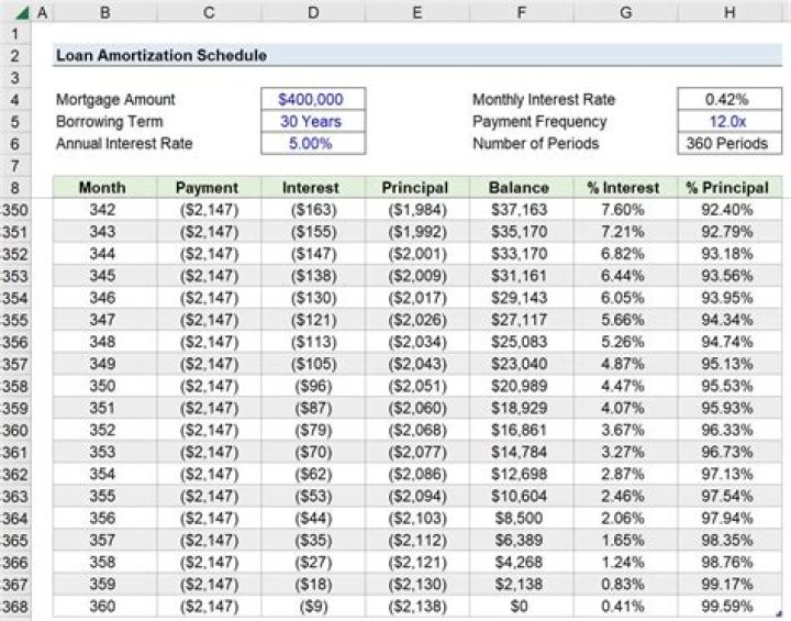
Loan Amortization Schedule
- Use the PPMT function to calculate the principal part of the payment.
- Use the IPMT function to calculate the interest part of the payment.
- Update the balance.
- Select the range A7:E7 (first payment) and drag it down one row.
- Select the range A8:E8 (second payment) and drag it down to row 30.
What is a loan payoff schedule called?
What Is an Amortization Schedule? An amortization schedule is a complete table of periodic loan payments, showing the amount of principal and the amount of interest that comprise each payment until the loan is paid off at the end of its term.
What is a payment schedule called?
Key Takeaways. An amortization schedule is a table that shows each periodic loan payment that is owed, typically monthly, and how much of the payment is designated for the interest versus the principal.
How does a projected loan payment schedule work?
The ‘Projected’ tab shows the expected payment schedule assuming the borrower pays the minimum payment on time each month. The loan fully amortizes as of the end of the loan term. In essence, this tool is two basic amortization tables with a slight adjustment on the Actual tab to allow for tracking.
How to create a date accurate payment schedule?
This calculator will solve for any one of four possible unknowns: “Amount of Loan”, “Total Scheduled Periods” (term), “Annual Interest Rate” or the “Periodic Payment”. Enter a ‘0’ (zero) for one unknown value. The term (duration) of the loan is a function of the “Total Scheduled Periods” and the “Payment Frequency”.
Can you use a paid premium loan payback template?
You can use these paid, premium payment and free download loan payback templates to manage your various loans and their respective payment schedules in an orderly manner so that you never miss a deadline again. You can also see Amortization Schedule Template.
How to create a loan repayment schedule in Excel?
To create a loan schedule, we will use the different formulas discussed above and expand them over the number of periods. In the first period column, enter “1” as the first period and then drag the cell down. In our case, we need 120 periods since a 10-year loan payment multiplied by 12 months equals 120.